As you saw before, Python is not statically typed, i.e. variables can change their type on the fly:
a =5a ='apple'print(a)
This makes Python very flexible. Out of these variables you form 1D lists, and these can be inhomogeneous:
a = [1, 2, 'Vancouver', ['Earth', 'Moon'], {'list': 'an ordered collection of values'}]
a[1] ='Sun'a
Python lists are very general and flexible, which is great for high-level programming, but it comes at a cost. The
Python interpreter can’t make any assumptions about what will come next in a list, so it treats everything as a generic
object with its own type and size. As lists get longer, eventually performance takes a hit.
Python does not have any mechanism for a uniform/homogeneous list, where – to jump to element #1000 – you just take
the memory address of the very first element and then increment it by (element size in bytes) x 999. Numpy library
fills this gap by adding the concept of homogenous collections to python – numpy.ndarrays – which are
multidimensional, homogeneous arrays of fixed-size items (most commonly numbers).
This brings large performance benefits!
no reading of extra bits (type, size, reference count)
no type checking
contiguous allocation in memory
numpy lets you work with mathematical arrays.
Lists and numpy arrays behave very differently:
a = [1, 2, 3, 4]
b = [5, 6, 7, 8]
a + b              # this will concatenate two lists: [1,2,3,4,5,6,7,8]
importnumpyasnpna = np.array([1, 2, 3, 4])
nb = np.array([5, 6, 7, 8])
na + nb # this will sum two vectors element-wise: array([6,8,10,12])na * nb # element-wise product
Working with mathematical arrays in numpy
Numpy arrays have the following attributes:
ndim = the number of dimensions
shape = a tuple giving the sizes of the dimensions
size = the total number of elements
dtype = the data type
itemsize = the size (bytes) of individual elements
nbytes = the total memory (bytes) occupied by the ndarray
strides = tuple of bytes to step in each dimension when traversing an array
np.arange(11,20) # 9 integer elements 11..19np.linspace(0, 1, 100) # 100 numbers uniformly spaced between 0 and 1 (inclusive)np.linspace(0, 1, 100).shape
np.zeros(100, dtype=np.int) # 1D array of 100 integer zerosnp.zeros((5, 5), dtype=np.float64) # 2D 5x5 array of floating zerosnp.ones((3,3,4), dtype=np.float64) # 3D 3x3x4 array of floating onesnp.eye(5) # 2D 5x5 identity/unit matrix (with ones along the main diagonal)
You can create random arrays:
np.random.randint(0, 10, size=(4,5)) # 4x5 array of random integers in the half-open interval [0,10)np.random.random(size=(4,3)) # 4x3 array of random floats in the half-open interval [0.,1.)np.random.rand(3, 3) # 3x3 array drawn from a uniform [0,1) distributionnp.random.randn(3, 3) # 3x3 array drawn from a normal (Gaussian with x0=0, sigma=1) distribution
Indexing, slicing, and reshaping
For 1D arrays:
a = np.linspace(0,1,100)
a[0] # first elementa[-2] # 2nd to last elementa[5:12] # values [5..12), also a numpy arraya[5:12:3] # every 3rd element in [5..12), i.e. elements 5,8,11a[::-1] # array reversed
Similar for multi-dimensional arrays:
b = np.reshape(np.arange(100),(10,10)) # form a 10x10 array from 1D arrayb[0:2,1] # first two rows, second columnb[:,-1] # last columnb[5:7,5:7] # 2x2 block
a = np.array([1, 2, 3, 4])
b = np.array([4, 3, 2, 1])
np.vstack((a,b)) # stack them vertically into a 2x4 array (use a,b as rows)np.hstack((a,b)) # stack them horizontally into a 1x8 arraynp.column_stack((a,b)) # use a,b as columns
Vectorized functions on array elements (a.k.a. universal functions = ufunc)
One of the big reasons for using numpy is so you can do fast numerical operations on a large number of elements. The
result is another ndarray. In many calculations you can use replace the usual for/while loops with functions on
numpy elements.
a = np.arange(100)
a**2# each element is a square of the corresponding element of anp.log10(a+1) # apply this operation to each element(a**2+a)/(a+1) # the result should effectively be a floating-version copy of anp.arange(10) / np.arange(1,11) # this is np.array([ 0/1, 1/2, 2/3, 3/4, ..., 9/10 ])
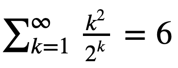
Exercise: Let’s verify the equation
using summation of elements of an ndarray.
Hint: Start with the first 10 terms k = np.arange(1,11). Then try the first 30 terms.
An extremely useful feature of ufuncs is the ability to operate between arrays of different sizes and shapes, a set of
operations known as broadcasting.
a = np.array([0, 1, 2]) # 1D arrayb = np.ones((3,3)) # 2D arraya + b # `a` is stretched/broadcast across the 2nd dimension before addition;# effectively we add `a` to each row of `b`
In the following example both arrays are broadcast from 1D to 2D to match the shape of the other:
a = np.arange(3) # 1D row; a.shape is (3,)b = np.arange(3).reshape((3,1)) # effectively 1D column; b.shape is (3, 1)a + b # the result is a 2D array!
Numpy’s broadcast rules are:
the shape of an array with fewer dimensions is padded with 1’s on the left
any array with shape equal to 1 in that dimension is stretched to match the other array’s shape
if in any dimension the sizes disagree and neither is equal to 1, an error is raised
Example 1:
==========
a: (2,3)  ->  (2,3)  ->  (2,3)
b: (3,)   ->  (1,3)  ->  (2,3)
                                ->  (2,3)

Example 2:
==========
a: (3,1)  ->  (3,1)  ->  (3,3)
b: (3,)   ->  (1,3)  ->  (3,3)
                                ->  (3,3)

Example 3:
==========
a: (3,2)  ->  (3,2)  ->  (3,2)
b: (3,)   ->  (1,3)  ->  (3,3)
                                ->  error
"ValueError: operands could not be broadcast together with shapes (3,2) (3,)"
Note on numpy speed: Not so long ago, I was working with a spherical dataset describing Earth’s mantle convection. It
is on a spherical grid with 13e6 grid points. For each grid point, I was converting from the spherical (lateral -
radial - longitudinal) velocity components to the Cartesian velocity components. For each point this is a
matrix-vector multiplication. Doing this by hand with Python’s for loops would take many hours for 13e6 points. I
used numpy to vectorize in one dimension, and that cut the time to ~5 mins. At first glance, a more complex
vectorization would not work, as numpy would have to figure out which dimension goes where. Writing it carefully and
following the broadcast rules I made it work, with the correct solution at the end – while the total compute time
went down to a few seconds!
Let’s use broadcasting to plot a 2D function with matplotlib:
%matplotlib inline
importmatplotlib.pyplotaspltplt.figure(figsize=(12,12))
x = np.linspace(0, 5, 50)
y = np.linspace(0, 5, 50).reshape(50,1)
z = np.sin(x)**8+ np.cos(5+x*y)*np.cos(x) # broadcast in action!plt.imshow(z)
plt.colorbar(shrink=0.8)
Exercise: Use numpy broadcasting to build a 3D array from three 1D ones.
Aggregate functions
Aggregate functions take an ndarray and reduce it along one (or more) axes. E.g., in 1D:
a = np.linspace(1, 2, 100)
a.mean() # arithmetic meana.max() # maximum valuea.argmax() # index of the maximum valuea.sum() # sum of all valuesa.prod() # product of all values
a = np.linspace(1, 2, 100)
a <1.5a[a <1.5] # will only return those elements that meet the conditiona[a <1.5].shape
a.shape
More numpy functionality
Numpy provides many standard linear algebra algorithms: matrix/vector products, decompositions, eigenvalues, solving
linear equations, e.g.
a = np.array([[3,1], [1,2]])
b = np.array([9,8])
x = np.linalg.solve(a, b)
x
np.allclose(np.dot(a, x),b)    # check the solution
External packages built on top of numpy
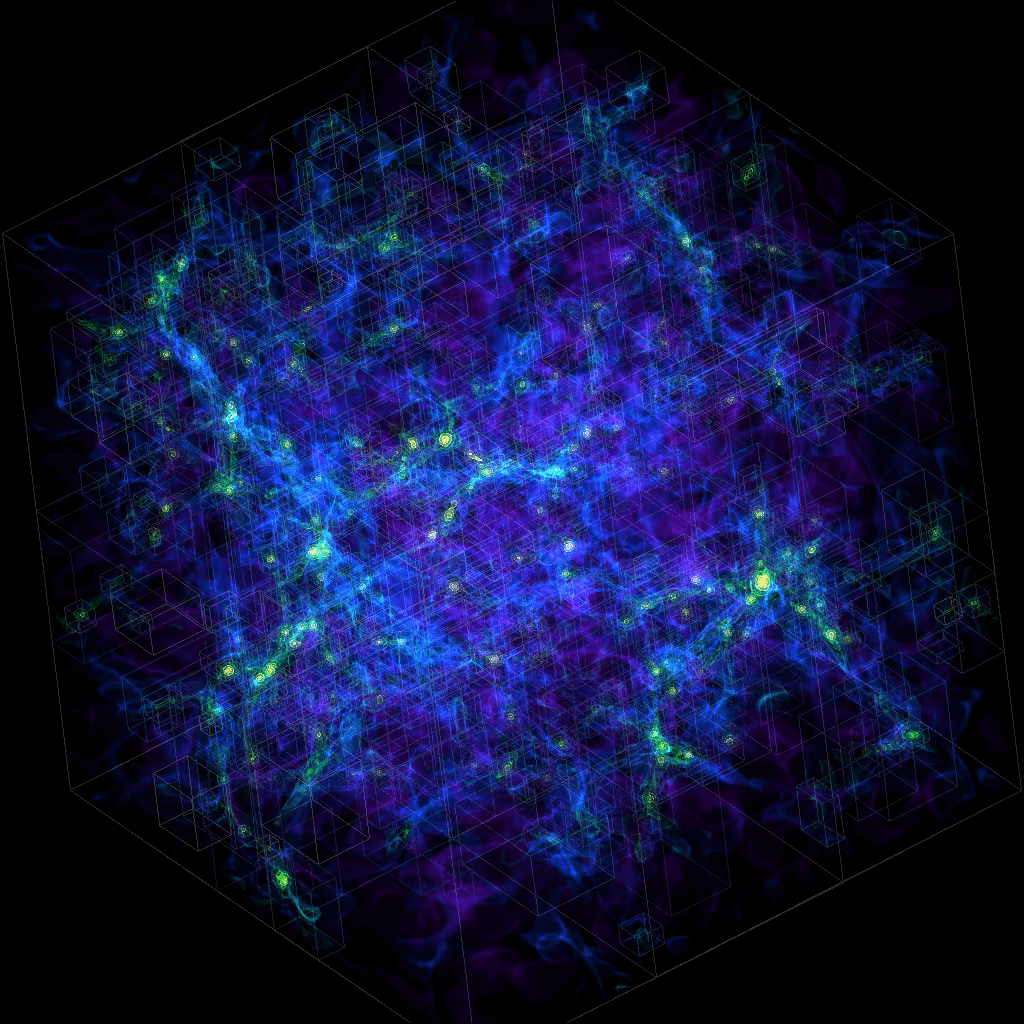
A lot of other packages are built on top of numpy. E.g., there is a Python package for analysis and visualization of 3D
multi-resolution volumetric data called yt which is based on numpy. Check out this
visualization produced with yt.
Many image-processing libraries use numpy data structures underneath, e.g.
importskimage.io# scikit-image is a collection of algorithms for image processingimage = skimage.io.imread(fname="https://raw.githubusercontent.com/razoumov/publish/master/grids.png")
image.shape # it's a 1024^2 image, with (R,G,B,\alpha) channels
Another example of a package built on top of numpy is pandas, for working with 2D tables. Going further, xarray
was built on top of both numpy and pandas. We will study pandas and xarray later in this workshop.